Minimizing Cost Functions
- We saw that there is an analytical solution to minimize
- so we can just calculate the optimal parameters
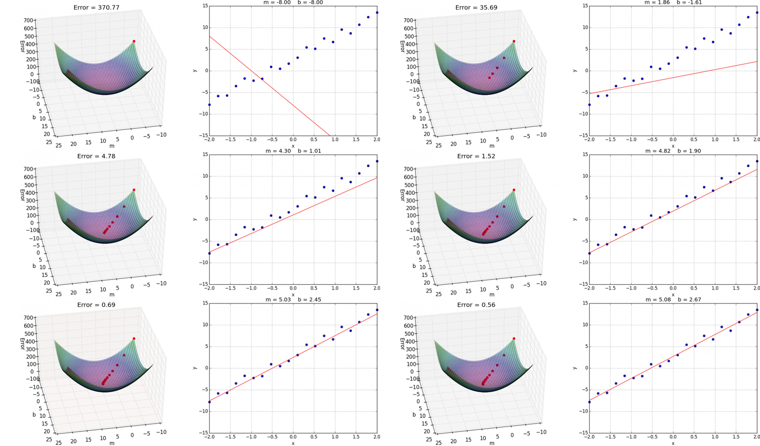
- But we could also calculate the result of the cost function for different parameter values to approach a minimum in the cost function

https://medium.com/analytics-vidhya/cost-function-explained-in-less-than-5-minutes-c5d8a44b918c
 Minimizing Complex Cost Functions
- ... parameters in a model, that is no linear regression (think )
- ... cost function in any machine learning model (think )

https://medium.com/analytics-vidhya/cost-function-explained-in-less-than-5-minutes-c5d8a44b918c
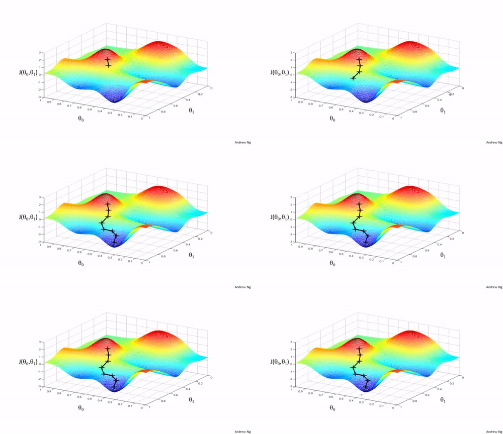
- We aim to find a global minimum
- How can we do this?
Gradient Descent Heuristic
- Start at a random position in the cost function
- Calculate the slope of the cost function at the current position
- If the slope is negative, move to the right
- Repeat
- Example with only one parameter (
theta) - and only one local minimum of the cost function that is the global minimum, where
start at random position theta in the cost function

while J'(theta)>0:
    Calculate the slope of J: J'(theta) at the current position
    If slope is negative:
        move theta to right by step width alpha
    If slope is positive:
        move theta to left by step width alpha
- the step with is called learning rate
Gradient
- more dimensional derivative
- gives us the direction of the steepest incline
- which weight has the biggest influence on the cost
- with only one
Example with a single
-
Example data
Data points: and
, -
We want to fit a line with no intercept
-
we can write down the cost function:
-
we can calculate the derivative
- what if we use flat line ()
- We make a large error ()
- The slope is negative (), so we must increase
- what if we use use line with incline of ()
- We make a much smaller error ()
- The slope is positive (), so we must decrease
 Key Takeaways
- if we have any cost function (error measure) that is derivable, we have an algorithm to estimate "good" parameters
- this algorithm converges on a local minimum of the cost function, depending on the starting parameters
- we are not guaranteed to find a global minimum
https://www.fromthegenesis.com/gradient-descent-part1/
Teaching Computers
- Machine Learning is about teaching computers to learn from data
- In many cases, we want to minimize the error of a model
- Gradient Descent is a general algorithm to minimize errors
- There are many variations of Gradient Descent
 Learning Rates
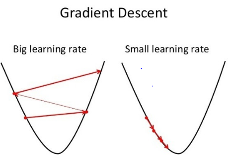
- the slope/gradients shows the direction but, we must decide for a step width (learning rate )
- Learning rate is too big: We can overshoot the target
- Learning rate is too small: Slow learning

https://www.fromthegenesis.com/gradient-descent-part1/
 Improvement: Adaptable Learning Rates
- Steps are larger in steeper areas
- Steps get smaller over time
https://wiki.tum.de/display/lfdv/Adaptive+Learning+Rate+Method?preview=/23573655/25008837/perceptron_learning_rate local minima.png
 Other Improvements
- Momentum strategy - consider direction of the last steps
- Stochastic Gradient Descent - Jump Around based on a subset of training data!

https://www.researchgate.net/publication/2295939_Lecture_Notes_in_Computer_Science/figures?lo=1
When to stop learning?
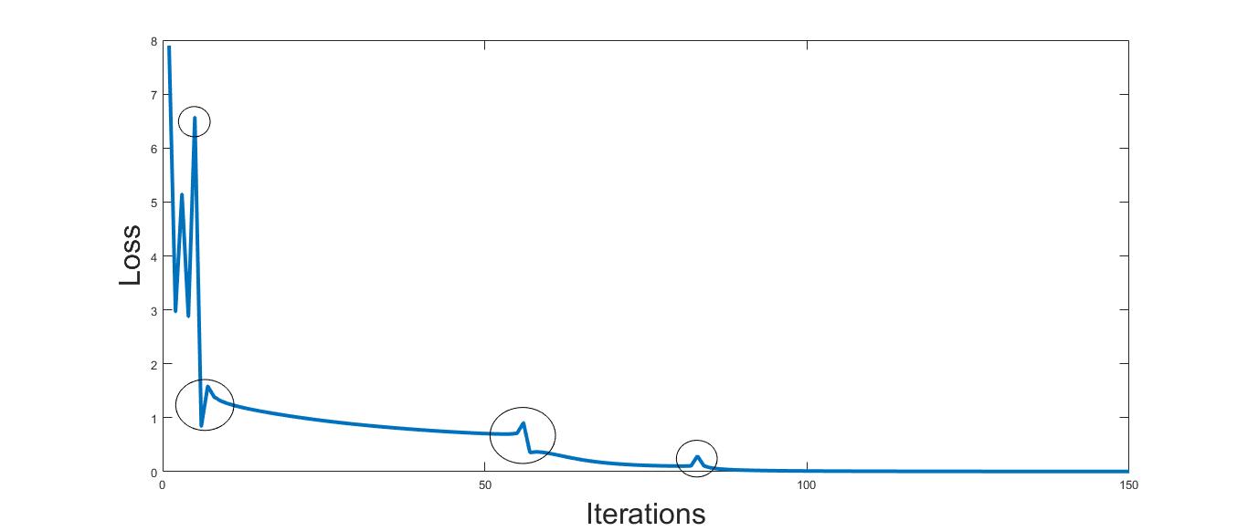
- Learning Curves plot the development of the training error over the steps (iterations of gradient descent)

- The loss (value of the cost function ()) will never be zero
- except for a perfect (over)fit on the training data
 Solution: Stopping criteria
- maximum number of iterations
- early-stopping: no (big) improvement for iterations
https://ai.stackexchange.com/questions/22369/why-the-cost-loss-starts-to-increase-for-some-iterations-during-the-training-pha
Different Learning Algorithms
- for different machine learning models use different algorithms
- almost all follow the basic principle of gradient descent
- they can differ in both speed and accuracy
- take the default or test them during model selection
https://machinelearningmastery.com/adam-optimization-algorithm-for-deep-learning/#:~:text=Adam is a replacement optimization,sparse gradients on noisy problems.
 Task
Task
-
Next, we look into an implementation of gradient descent
-
Homework: 6.1 Learning and Accuracy Functions - Gradient Descent
-
In class: 6.2 Gradient Descent in Python
2.6.2 Accuracy Measures and Learning Curves
 Learning objectives
You will be able to
- use different accuracy measures
- use learning curves to identify over-fitting
What is a good model?
- A good model makes an accurate prediction
- Models with a low flexibility (high bias) are not accurate because they are too simple do model the real world
- Models with a high flexibility (high variance) are not accurate because they are too complex and overfit the training data
https://medium.com/@ivanreznikov/stop-using-the-same-image-in-bias-variance-trade-off-explanation-691997a94a54
 Cost and Accuracy Measures
- Residual Sum of Squares
- Squared error for the whole data set with observations
- Mean Squared Error
- Squared error for the average observation
- Root Mean Squared Error
- corrected for the dimension
https://scikit-learn.org/stable/modules/classes.html#regression-metrics
-
Mean Absolute Error
- keeps the unit of the predicted variable
-
Mean Absolute Percentage Error
- allows comparison between different data sets
- not defined for , biased for small
 Learning Curves
- A learning curve is a plot of model learning performance over experience or time (e.g., number of iterations of gradient descent or amount of training data).
- To really understand how a model behaves, the data must be split in a training an validation set
- Training Learning Curve: Learning curve calculated from the training dataset that gives an idea of how well the model is learning
- Validation Learning Curve: Learning curve calculated from a hold-out validation dataset that gives an idea of how well the model is generalizing
https://machinelearningmastery.com/learning-curves-for-diagnosing-machine-learning-model-performance/
The Learning Curve Plot
- Learning Curve: Line plot of learning (y-axis)
- Loss/Score can be any accuracy measure
- over experience (x-axis).
- for instance number of iterations
- size of the training set
- duration of training
https://upload.wikimedia.org/wikipedia/commons/2/24/Learning_Curves_(Naive_Bayes).png
 Examples
- Model too flexible and over-fits the data
- small training error but large validation error
 Examples
- Model is flexible, but training was stopped to early
- We would expect a better fit with more training
 Examples
- Model is very flexible and over-fits the training data
- after some time so the loss on unseen validation data increases a little
 Examples
- Example for a good fit
- Usually we would expect a better fit on the training set than the validation set
 Examples
- Training set might be to small
- Data fits the training set well but this does not translate to the validation set
 Examples
- Validation set might be to small
- Depending on the selection of the values in the set the loss fluctuates a lot (high variance)
 Case Study
- we train different model on synthetic data set
- we use training curve, to see how the models behave during training
6.3 Accuracy Measures and Learning Curves
25 min