2.4 Multiple Regression

2.4.1 Multiple Linear Regression

Learning objectives

You will be able to

• implement and interpret Linear Regression models with multiple independent variables
• Students can calculate the VIF to remove colinear predictors
• name different approaches for variable selection

Need für Multiple Regression

How do the total sales relate to the three different advertising budgets?

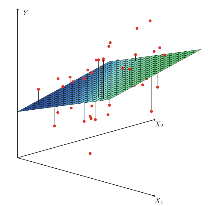
Interpreting Multiple Regression

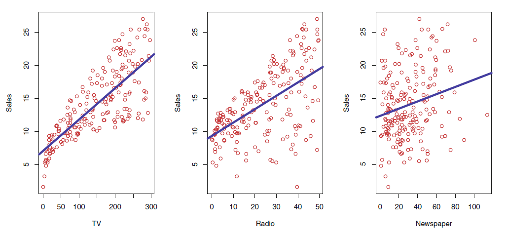
• only newspaper adds show no significant correlation to sales

Take care when comparing different models

• If we only consider newspaper adds, they have a significant correlation
• the single equation ignores the other two media in forming estimates for the regression coefficients.

Visualization

2.4.2 Variable Selection

• which predictors should we include in the model?
  • $\text{sales} = β_0 + β_1 × \text{TV} + β_2 × \text{radio} + β_3 × \text{newspaper} + \epsilon$
  • $\text{sales} = β_0 + β_1 × \text{TV} + β_2 × \text{radio} + \epsilon$
  • $\text{sales} = β_0 + β_1 × \text{TV} + β_3 × \text{newspaper} + \epsilon$
  • $\text{sales} = β_0 + β_2 × \text{radio} + β_3 × \text{newspaper} + \epsilon$
  • $\text{sales} = β_0 + β_1 × \text{TV} + \epsilon$
  • $\text{sales} = β_0 + β_2 × \text{radio} + \epsilon$
  • $\text{sales} = β_0 + β_3 × \text{newspaper} + \epsilon$

Model Selection

• there are $2^p$ models that contain subsets of $p$ variables.
• there are different criteria for model quality ($MSE$, $R^2$, ...)
• Approaches:
  • Forward selection: Start with null model (only intercept $\beta_0$) and add variables
  • Backward selection: Start with all variables and remove variables
• More in the next session

Collinearity

• two or more predictor variables are closely related to one another
• makes difficult to separate out the individual effects
• reduces the accuracy of the estimates of the regression coefficients
• You can spot them in scatter plot matrices

https://medium.com/analytics-vidhya/new-aspects-to-consider-while-moving-from-simple-linear-regression-to-multiple-linear-regression-dad06b3449ff

Variance inflation factor (VIF).

• Even better: compares how much a variable $j$
  adds the to problem
  $VIF_j=\frac{1}{1-R_j^2}$

• The smallest possible value for VIF is 1,
  which indicates the complete absence
  of collinearity.

• $VIF > 5 \text{ or } 10$ indicates a problematic amount of collinearity.

• What to do:

  • Check VIF for all possible predictors
  • drop the predictor with the highest $VIF$

$R_j^2$ is the result of regressing $j$ on all other predictors

Case Study

If we would like to create a model, that predicts the flipper length not only from bill length but also bill depth, we need to define a model with multiple predictors.

https://www.scoopnest.com/user/AFP/1035147372572102656-do-you-know-your-gentoo-from-your-adelie-penguins-infographic-on-10-of-the-world39s-species-after

Case Study

4.1 Multiple Linear Regression

25 minutes

2.4.3 Qualitative Predictors and further Extensions

Learning objectives

You will be able to

• integrate qualitative predictors in regression models
• model non-linear relationships with linear regression
• name common problems when working with linear regression

Qualitative Predictors

• so far the models only included quantitative (interval scaled) predictors

• how do we deal with qualitative data

Predictors with only Two Levels

• $x_{1,j}$ femur length of person $j$

• $x_{2,j} = \begin{cases} 1 & \text{if jth person is female} \\ 0 & \text{if jth person is male} \end{cases}$

Interpretation of $\beta_2$

• if $\beta_2$ is negative:
  • a woman will be shorter with the same femur length

Qualitative Predictors with more than two Levels

• if the data contains the following ethnicities: Asian, Caucasian, African American
• we would need two additional variables:

• in the models base line, the person is African American so $x_3 = x_4 = 0$

Example: Input Features that are not numerical

• most models only can work with numerical variables

Dummy Encoding

• $n-1$ new variables for each category in the original variable
• there is a baseline model (e.g., is male and african american)
• common in linear regression

One-Hot Encoding

• $n$ new variables for each category in the original variable
• common in other machine learning models

Example of a Regression Table with Dummy Encoding

• the only predictor in $X$ is ethnicity (three classes)
• the baseline is African American, where the intercept (predicted value $Y$ is $531$)
• for both other ethnicity, the model expects a lower value
• however, the correlation is not significant ($p>0.05$)

Case Study

4.2 Applications of Linear Regression

2.4.4 Extensions of the Linear Model

• Linear Regression is a simple, yet powerful tool
  • it's the go-to tool in research to evaluate correlation in data
  • it's a commonly used model a a baseline for more sophisticated models
• There are two common extensions, that make it even more powerful

Removing the Additive Assumption

In reality, is it better to spent all the marketing budget on TV or to split it?

• this model is purely additive

• we assume the effects on the sales to be independent
• in reality, we expect synergies (e.g, when people see the add twice)

by adding Interaction Terms

• We can model this, using an interaction term ($\text{TV} × \text{radio}$)

• Interpretation: There is an additional positive effect, if we increase both
  (TV and radio adds)

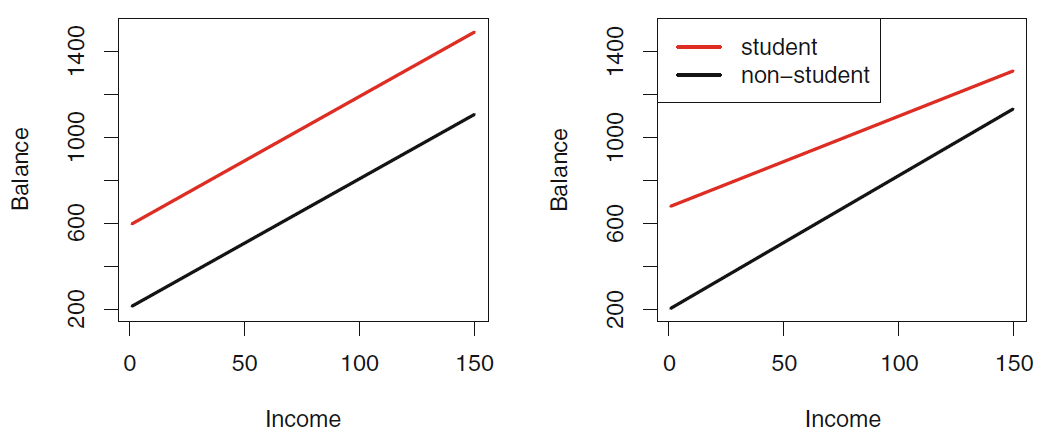
Interactions with qualitative Predictors

prediction of bank account balance from income

• Left Model:

• Right Model:

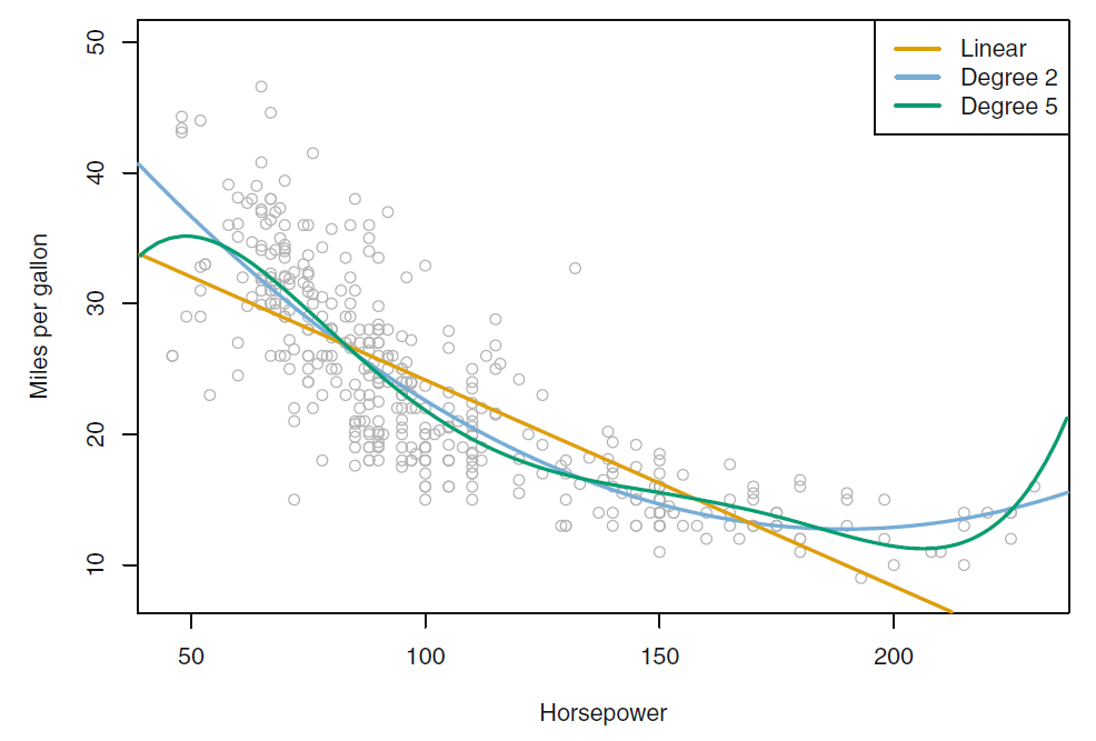
Modeling non-linear Relationships with Linear Models

the linear model is no good predictor for the relationship

Linear Regression Model can capture non linear Relationships

• polynomial regression:

• Drawbacks
  • we have to decide for the degree of the polynom (parametric model)
  • it is harder to interpret
  • there are more flexible models

Case Study: Data Science Project with Linear Regression

Imagine researching penguin in the Antarctic caused Your scale to freeze an break. However, You still want to get an estimate of the penguins weight.

Luckily, Your colleagues left You with a data set (train) with all the other variables you can measure.

Create a multiple linear regression model to predict the penguins weight. Compare the Mean Squared Error of the model in the test set with your colleagues.

https://www.scoopnest.com/user/AFP/1035147372572102656-do-you-know-your-gentoo-from-your-adelie-penguins-infographic-on-10-of-the-world39s-species-after

4.3 Case Study

45 minutes