2.2 Statistical Learning

2.2.1 Basics of Statistical Learning

Learning objectives

You will be able to

• categorize problems in supervised and unsupervised learning
• differentiate problems of prediction and interpretation
• explain the purpose of a training and test set

Definitions

• Data Science or Statistical Learning refers to a vast set of tools for understanding data
• supervised statistical learning involves building a statistical model for predicting,
  or estimating, an output based on one or more inputs

https://www.finbridge.de/data-science

Example Supervised: Wage Data (Input and Output)

• How does output $Y$ (wage) relate to input $\vec{X}$ (age, year, education)

[Hasties]

A Brief History of Statistical Learning

• 1800s Legendre and Gauss: Linear Regression
• 1970s Generalized
  linear models (non-linear relationships was computationally infeasible)
• 1980s Classification and
  regression trees
• 2000s Machine Learning

https://zakharus.medium.com/data-science-timeline-305ef75dceb6

1800s Legendre and Gauss: Linear Regression

• describing the relation between two variables with the best fitting curve

1870-1970s Classical Statistics

• formalized statistical test
• t-test e.g., William Sealy Gosset's 1908 paper in Biometrika working for Guinness Brewery

2000s Machine Learning

• complex data points (sentences, images, DNA-sequences)
  instead of numeric variables
• models with "uncountable" parameters, fitted to the data with computing power

https://www.medrxiv.org/content/10.1101/2020.07.17.20155150v1.full

2010s "Artificial Intelligence"

• deep neural networks (efficient matrix multiplication on GPUs)
• Generative Adversarial Networks that learn to produce
• Reinforcement Learning

https://openai.com/dall-e-2/

Structure of Supervised Learning Problems

• model ($f$) describes how one or many predictors ($\vec{X}$)
  relate to a predicted variable $Y$: $f(\vec{X}) = Y$

Nomenclature

• $\vec{X}$ input variables (predictors, independent variables, features)
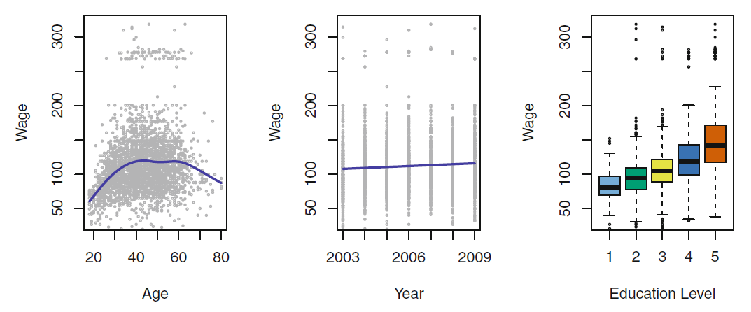
  • e.g, age, years on the job, education
• $Y$ output variable (response or predicted/dependent variable)
  • e.g., income

we use large letters, when we speak about the random variable, [Hasties]

• We assume that there is some relationship between $Y$ and and $p$ different predictors, $\vec{X}= X_1,X_2, . . .,X_p$.

• $f$ is a fixed but unknown function of $X_1, . . . , X_p$,
• $\epsilon$ is a random error term, which is independent of $\vec{X}$ and has mean zero.
• $f$ represents the systematic information that $\vec{X}$ provides about $Y$

Applications

• Why estimate $f$?
• we build models to
  • predict the future
    what should we offer out next employee?
  • understand the world (interpretation)
    should it do a master?

Prediction

• We want to make a prediction about
  • the future - stock prices
  • an unknown property - does the patient have cancer?

1. • a hat symbol ( $\hat{}$ ) indicates a prediction
   • $\hat{f}$ is often a black box, in machine learning the model is a prediction based on the data
   • We probably make an prediction error $\epsilon$
   • We are interested in the accuracy of $\hat{Y}$

Prediction Example

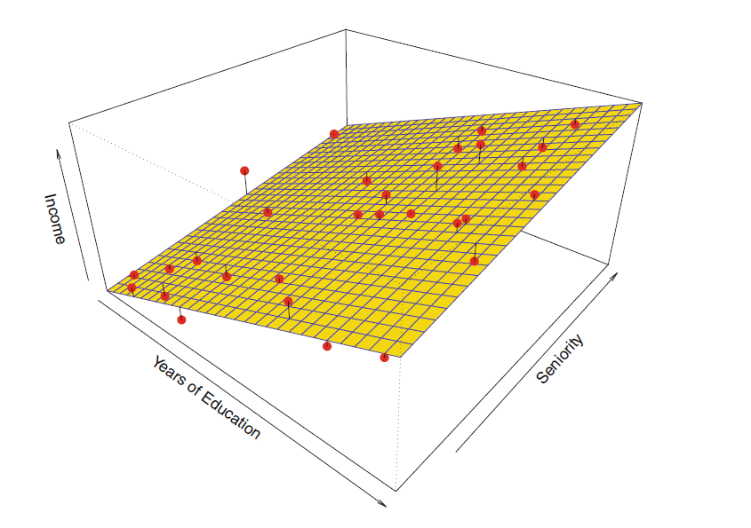
• Can we predict the income based on the
  education and years of seniority in the job

• the model $\hat{f}$ is the blue area
• we can plug in eduction ($X_1$) and seniority ($X_2$)
• to get an prediction on the income ($\hat{Y}$)
• we do not care what $\hat{f}$ looks like as long we make small errors $\epsilon$ for each observation (red dot)

[Hasties]

Interpretation

• how is $Y$ affected as $X_1, . . . , X_p$ change?
• $\hat{f}$ must not be a black box, because we need to know its exact form
• We are interested in the parameters $\beta_0, \beta_1, . . . , \beta_p$ of the model
• How strong is the relationship between the response and each predictor?
  • How much more will a person earn for each year of education?
• Which predictors are associated with the response?
  • Does seniority have any impact at all?
• Can the relationship between $Y$ and each predictor be adequately summarized
  using a linear equation, or is the relationship more complicated?
  • Will the income increase in a stable way?
  • Is there a safe level of alcohol consumption?

Interpretation or prediction?

• : prediction
• : interpretation

• What's the gas price next summer?
• Do students in the front row get better grades?
• Given an x-ray picture, does the patient have lung cancer?
• What has the lager influence on weight: sugar or fat intake?

How do we estimate $f$?

• training data ($n$ observations of our sample, rows in a table) to train, or teach, our method how to estimate $f$
  (e.g., income based in education and seniority)
• $x_{i,j}$
  • the value of the $j$th of $p$ predictors
  • for observation $i$ of $n$ observations
  • where $j = 1, 2, . . ., p$ and $i = 1, 2, . . . , n$.
• $\vec{x}_i = (x_{i,1}, x_{i,2}, . . . , x_{i,p})^T$
  • We use the small $\vec{x}_i$ to indicate the vector of all predictors of observation $i$ (i.e., a row)
• $X_j= (x_{1,j}, x_{2,j}, . . . , x_{n,j})$
  • We use the capital $X_j$ to indicate the vector of the $n$ values of the $j$th predictor (i.e., a column)

• $y_i$ response variable for the $i$th observation.
• Then our training data consist of
  ${(\vec{x}_1, y_1), (\vec{x}_2, y_2), . . . , (\vec{x}_n, y_n)}$
• Our goal is to apply a statistical learning method to the training data
  in order to estimate the unknown function $f$.
• so that $y_j ≈ \hat{f}(\vec{x}_j)$ for any observation $i$.
• There are parametric and non-parametric methods (compare blue planes in the prediction example)

2.2.2 Parametric and non-parametric Models

Learning objectives

You will be able to

• differentiate parametric and non-parametric models
• calculate accuracy measures of regression models
• interpret in (training-set) and out-of-sample (test-set) accuracy in terms of model flexibility, bias, variance, and over-fitting

Parametric Methods

• Step 1: assumption about the functional form or shape of $f$.

  • e.g., a simple linear form
    $f(\vec{X}) = β_0 + β_1X_1 + β_2X_2 + ... + β_pX_p.$

• Step 2: training data to fit the model.

  • we need to estimate the parameters $β_0, β_1, . . . , β_p$.
  • find values of these parameters such that
    $Y ≈ β_0 + β_1X_1 + β_2X_2 + . . . + βpXp.$

$X_i:$ Variable $i$

Parametric model of income explained by years of education and years on the job (seniority)

Matrix Representation for Linear Models

• $x_{i,j}$… value of predictor $j$ of observation $i$
• $X_0=x_{:,0}$… are all $1$ so $x_{j,0} \cdot \beta_0 = \beta_0$ is the bias term
  (i.e., the intercept of the linear regression model)

$\text{income} ≈ β_0 + β_1 \cdot \text{education}+ β_2 \cdot \text{seniority}$

• Observation 1
  • $y_1=\beta_0 + \beta_1 \cdot x_{1,1} + \beta_2 \cdot x_{1,2}$
  • $40.000=\beta_0 + \beta_1 \cdot 10 + \beta_2 \cdot 1$
• Observation 2
  • $y_2=\beta_0 + \beta_1 \cdot x_{2,1} + \beta_2 \cdot x_{2,2}$
  • $50.000= \beta_0 + \beta_1 \cdot 13 + \beta_2 \cdot 4$

Parametric Methods

• $\text{income} ≈ β_0 + β_1 × \text{education}+ β_2 × \text{seniority}$
• form is fixed, but we can tweak three parameters to improve the fit ($β_0, β_1, β_2$)
• $β_0$ is the intercept

• $\beta_0$: uneducated workers without eduction get a salary of $20.000\text{ €}$

• $\beta_1$: one year of education results in $1.500\text{ €}$ higher salary

• $\beta_2$: one year of working experience results in $1.000\text{€}$ higher salary

• linear regression is a parametric and relatively inflexible approach

  • it can only generate linear functions
  • only two factors (lines) to interpret

Task

2.1 Storing $Y$ and $X$ in a DataFrame

Non-parametric Methods

• no explicit assumption about the functional form of $f$
• but some kind of algorithm of $f$
  • close to the data points
  • without being too rough or wiggly
• e.g., a hand-drawn line is a non-parametric model

Over-fitting

• more common with flexible, non-parametric methods
• perfect prediction for any point in the training data
• probably not a good prediction for points that are not in the training data

Sample split in Training and Test Set

• Training data: the data we use for building the mode (e.g., finding /fitting the right parameters for the model)
• Test data: Hold-out sample, that we can use to test how well the model performs on unseen data
  • more important with prediction tasks

Trade-Off Between Prediction Accuracy and Model Interpretability

• parametric models are usually easier to interpret

Which to use for prediction and interpretation?

• Non-parametric model tend to be more powerful
  and therefore better for predictions
• Parametric models are less flexible but have
  clear parameters ($\beta$ sometimes called $\theta$) that are
  easier to understand for interpretation

Task

2.2 Creating a Training and Test set

Assessing Model Accuracy

• There is no free lunch in statistics:
  no one method dominates all others over all
  possible data sets.

• How to decide for any given set of data which method produces the best results?

https://xkcd.com/2048/

Measuring the Quality of Fit

• the error of each prediction $e_j$ tells us how well the predictions match the observed data

• Mean squared error ($\text{MSE}$) is a common accuracy measure,

Training vs Test Set

• Many methods minimize the $\text{MSE}$ during training (training $\text{MSE}$, in-sample $\text{MSE}$)
• in general, we do not really care how well the method works during training on the training data,
• but how our methods works on previously unseen test data (out-of-sample $\text{MSE}$)

Fitting Data with a low flexibility Model

• $f_{\text{low}}(x)=\hat{y}(x)=\beta_0$

  • (i.e., the mean of all red dots of the training data)
  • only one parameter $\beta_0$

• black: prediction

• red: Training data (medium fit)

• blue: Test data (good fit)

Fitting Data with a medium flexibility Model

• $f_{\text{med}}(x)=\hat{y}(x)=\beta_0 + \beta_1 \cdot x$

  • two parameters $\beta_0$ and $\beta_1$

• black: prediction

• red: Training data (good fit)

• blue: Test data (good fit)

Fitting Data with a high flexibility Model

• $f_{\text{high}}(x)=\hat{y}(x)\\=\beta_0 + \beta_1 \cdot x + \beta_2 \cdot x^2$
  • three parameters $\beta_0$, $\beta_1$, $\beta_2$
• black: prediction
• red: Training data (very good fit)
• blue: Test data (poor fit)

Task

2.3 Training Models on a Test Set

The Bias-Variance Trade-Off and Over-Fitting

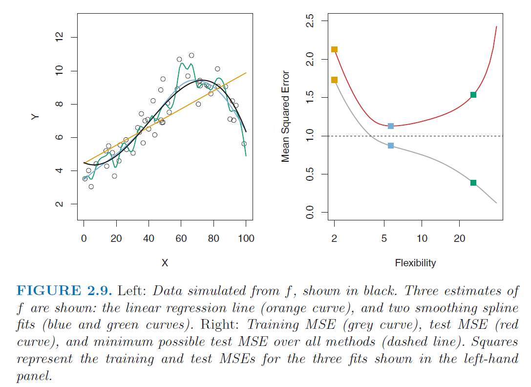
• The higher the flexibility
  • the lower the $MSE$ on the training data
  • the higher the $MSE$ on the test data

• U-shape in the test MSE is the result of two competing properties of statistical learning methods
• Variance refers to the amount by which $\hat{y}$ would change
  if we estimated it using a different training data set.
• Bias refers to the error that is introduced by approximating
  a real-life problem, which may be extremely complicated,
  by a much simpler model.

See Hasties p. 34 correct formula

• Black line: Error on the test set
• more flexible (complex, often non-parametric) models have higher variance but lower bias
• they can fit the data better (low bias), but are more influenced by the data (high variance)

Task

2.4 Preventing Non-Parametric Models from Over-Fitting